Linear regression in R and python

Fortunately (or unfortunately), I haven’t had the need to learn python in detail to carry out my main job functions. However, python has gained quite a lot of traction for data science and bioinformatics, thus I’ve decided to get up to speed during the few breaks I get.

Today I wanted to see how simple is to translate some very basic R code to python. Specifically, I wanted to see how to do the following in python:

• Work with data frames
• Simulate data
• Perform linear regressions
• Plot data

For this particular exercise I will create a data frame with simulated data drawn from a multivariate normal distribution for which I will know the real regression coefficients, and check these through a linear regression.

R code

In R, achieving this is very simple with the help of the MASS library. The code for a simple simulation and linear regression looked like this:

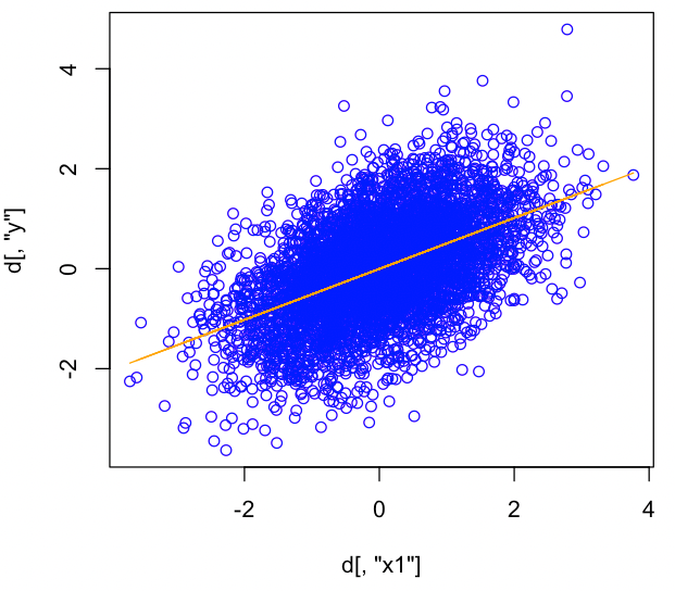
Briefly, in the snippet above, I first simulate some data using the function mvrnorm() that will draw random numbers from a multivariate distribution for two variables with mean=0, var(x1)=var(y)=1 and cov(y,x1)=0.5. The linear regression is then fit with the lm() function, and the summary() allows to inspect the results:

Coefficients:
            Estimate Std. Error t value Pr(>|t|)    
(Intercept) -0.00428    0.01229  -0.348    0.728    
x1           0.50926    0.01218  41.801   <2e-16 ***

Here we see that the regression coefficient for x1 = 0.509 which is in line with what we simulated b = cov(y,x1)/var(x1)=0.5/1=0.5

The data and regression line are then plotted with plot() and lines() function:

Code for a multivariable regression looks very similar, here I am adding an extra variable, changing the mean of my outcome variable y to mean=2 and assigning cov(y,x1)=0.4 and cov(y,x2)=0.2. Given that variances = 1 across variable, we expect the regression coefficients to be ~0.4 for x1 and ~ 0.2 for x2.

And the result:

....
Coefficients:
            Estimate Std. Error t value Pr(>|t|)    
(Intercept)  1.99545    0.01261  158.29   <2e-16 ***
x1           0.41296    0.01255   32.90   <2e-16 ***
x2           0.20444    0.01267   16.13   <2e-16 ***
....

Python code

The first time I googled “linear regression in python”, I got prompted to look into sklearn.linear_model.LinearRegression . Then I realized that it was an overkill to use the sklearn library for this particular exercise (gladly, because there were too many lines of code). However, turns out that the python code is very similar to that from R if you use the library statsmodels . The following code replicates what was done in R in the previous section:

And this is the result:

coef    std err          t      P>|t|      [0.025      0.975]
------------------------------------------------------------------------------
x1             0.5185      0.012     43.433      0.000       0.495       0.542

Which seemed fine until I realized that there was no estimate for the intercept! — Turns out that unlike R, adding the intercept in the regression is not the default functionality. This has to be added manually by including a constant to the predictors data frame:

After adding the constant to the data frame of predictors with sm.add_constant(d['x1']) now the linear regression returns the intercept estimate as well:

coef    std err          t      P>|t|      [0.025      0.975]
------------------------------------------------------------------------------
const          0.0057      0.012      0.471      0.638      -0.018       0.029
x1             0.5187      0.012     43.426      0.000       0.495       0.542

Finally, the example of a multivariable regression in R “translated” to python looks like this: